04. GPR Fracture & Cavity Mapping¶

This chapter covers the geophysical front end of the repository: the ground-penetrating-radar (GPR) processing chain that turns a raw B-scan into a fracture map, the surface fitting and uncertainty ladder that turn that map into a quantified keep-out volume, and the earthworks reducers that lift a bedrock surface out of the same picks. The subsystem lives under Quarry/Processing, Quarry/Ingestion, and Earthworks in the Core assembly, with seven Grasshopper adapters on the Frahan > Quarry ribbon. It is the geological front end that chapter 3 (Quarry Block-Cutting) forward-references: chapter 3 takes the fracture mesh as given input, and this chapter builds it (docs/thesis/chapters/03_quarry-blockcut.md:21-22).

The whole pipeline is pure managed code. There is no MathNet, no Python runtime, no native shim on the processing path; the FFT, the Hilbert transform, the kriging, and the error function are all in-tree. This is a deliberate constraint: the prototype that the C# Core mirrors was a Python/numpy/scikit-learn script, and the port to dependency-light managed code is what makes the chain installable beside the .gha without forcing scipy onto every machine (RadargramProcessor.cs:9-30, Kriging.cs:8-29). The derivations below reuse the mathematics validated in the submitted BoEGE paper (Murugean 2026), which this subsystem underlies.

The core physical model is the constant-velocity time-to-depth conversion. A GPR records two-way travel time $t$; with electromagnetic velocity $v$ in the rock, the reflector depth is

\[ v=\frac{c}{\sqrt{\varepsilon_r}},\qquad \mathrm{depth}=\frac{v\,t}{2}, \]

where $c=0.299792458\,\mathrm{m/ns}$ and $\varepsilon_r$ is the relative permittivity (marble $\varepsilon_r\approx9$, $v\approx0.10\,\mathrm{m/ns}$; granite $\varepsilon_r\approx6$, $v\approx0.12\,\mathrm{m/ns}$). Velocity is the single highest-leverage value in the whole chain because every depth scales with it linearly (RadargramProcessor.cs:27-28; GprPresets.cs:18-19). The [Algorithm] attribute on the front-end component states the model in one line: "v=c/sqrt(eps_r); depth=v*t/2. Energy E=|s+iH{s}|^2; fractures are high-E continuous reflectors, intact stone is low-E" (GprFractureExtractComponent.cs:43-45).

4.1 Ingestion and the file dispatcher¶

The single canvas-side entry point is GprFileReader.Load, which dispatches by extension to the format reader: CSV, SEG-Y (.sgy/.segy), MALA (.rd3), Sensors & Software pulseEKKO (.dt1), IDS GeoRadar (.dt), and GSSI (.dzt) (GprFileReader.cs:23-46). The proprietary Geoscanners AKULA .gsf format is explicitly not guessed: the reader raises a NotSupportedException that tells the user to convert to SEG-Y with GPRSoft or RGPR first, because the binary spec is closed (GprFileReader.cs:46-51). This is the bridge-not-guess posture: a wrong header guess on a proprietary container would silently corrupt the depth axis.

RadargramProcessor.ToGrid builds the regular [samples, traces] amplitude grid and recovers the true two-way sample interval $\mathrm{d}t$ in nanoseconds, velocity-independent, so the caller scales depth with the stone velocity rather than baking a velocity into ingest. It prefers the reader-supplied SampleIntervalNs; only when that is unknown does it fall back to recovering $\mathrm{d}t$ from the metres-per-sample step at vacuum velocity ($\mathrm{d}z=c\,\mathrm{d}t/2$) (RadargramProcessor.cs:42-75).

Originality. GprFileReader and the per-format readers are vendored-library / clean-room depending on the format: each reader implements a published or open binary spec (pulseEKKO DT1/HD is the public-domain USGS OFR 02-166 spec, Lucius and Powers 1999; SEG-Y is the SEG standard). The dispatcher itself is a thin switch and adds no algorithm. No proprietary spec is reverse-engineered.

4.2 The B-scan processing chain¶

RadargramProcessor.Run is the validated chain, mirroring the Python prototype stage for stage (RadargramProcessor.cs:334-357):

\[ \textsf{dewow}\to\textsf{bg-removal}\to\textsf{time-zero mute}\to\textsf{smooth}\to\textsf{t-gain}\to[\textsf{Stolt}\to\textsf{smooth}]\to\textsf{Hilbert energy}\to\textsf{smooth}\to\textsf{depth-equalize}. \]

The early stages are elementary 1-D filters: dewow is a high-pass running-mean subtraction that removes the low-frequency "wow" baseline drift (Dewow, :100-115); background removal subtracts the mean trace to kill horizontal banding and the direct air-wave (:152-163); the time-zero mute zeroes the air-wave / antenna-coupling band (:165-170); t-power gain multiplies by $(i\,\mathrm{d}t+1)^p$ to compensate spherical divergence and absorption (:172-182). Each box-mean uses an $O(\mathrm{len})$ running sum with numpy 'same' edge semantics so the C# output is bit-comparable to the prototype (BoxMeanSame, :83-98). The column operations are independent, so they run as deterministic Parallel.For with thread-local scratch (a fixed output partition makes the parallel result bit-identical to the serial loop, :104-114, :295-307).

Originality. The dewow / background / mute / gain / AGC primitives are clean-room standard GPR processing (Annan 2009; Neal 2004), implemented from published signal-processing definitions with no upstream code in the tree. The contribution is the validated ordering and parameterisation, not the filters.

4.2.1 The FFT and Hilbert transform (clean-room numerics)¶

The spectral stages need an exact-length forward and inverse transform that matches numpy.fft. The in-tree Fft is a radix-2 Cooley-Tukey transform (Cooley and Tukey 1965) for power-of-two lengths, with a Bluestein chirp-z fallback for arbitrary lengths so the 2-D Stolt migration and the Hilbert envelope operate on the exact sample and trace counts; zero-padding would shift the frequency grid and bias the migration (Fft.cs:30-94). The Bluestein plan (the chirp and the precomputed kernel spectrum) is length-only, so it is built once per distinct length and reused across every trace, the single biggest speed-up for the 986-same-length envelope loop (Fft.cs:96-149).

The instantaneous-energy attribute is the analytic-signal magnitude. For a real trace $s$, the analytic signal is $s+i\,\mathcal{H}\{s\}$, where $\mathcal{H}$ is the Hilbert transform; the instantaneous amplitude (envelope) is its magnitude and the instantaneous energy is the square:

\[ E(i,t)=\bigl|\,s(i,t)+i\,\mathcal{H}\{s\}(i,t)\,\bigr|^2. \]

The envelope is computed by the spectral method (Taner, Koehler and Sheriff 1979): forward-FFT the trace, apply the one-sided weighting $H=[1,2,2,\dots,2,1,0,\dots,0]$ that doubles the positive frequencies and zeroes the negatives, inverse-FFT, take the magnitude (AnalyticEnvelope, Fft.cs:159-185; HilbertEnergy, RadargramProcessor.cs:293-308). The physical reading is the literature consensus: a fracture or cavity is an impedance contrast that reflects strongly, while intact stone is the low-energy background (Porsani et al. 2006; Isakova 2021), so high instantaneous energy is the fracture proxy.

Originality. Fft is clean-room: a numerical method (radix-2 + Bluestein) is not copyrightable and the file says so (Fft.cs:16-18). The Hilbert-envelope attribute is the textbook Taner et al. (1979) complex-trace analysis, cited in the front-end [Algorithm] (GprFractureExtractComponent.cs:44).

4.2.2 Stolt f-k migration with half-velocity (original derivation)¶

Diffraction hyperbolae and dipping reflectors are mispositioned in the raw B-scan; migration collapses diffractions and moves dipping events to true position. The repository implements Stolt (1978) f-k migration in the exploding-reflector model. The key step is the constant-velocity dispersion relation that maps the recorded temporal frequency $\omega$ to the vertical wavenumber $k_z$.

Derivation. A monochromatic plane wave in the exploding-reflector model travels at the migration velocity $v_m=v/2$ (the half-velocity that converts two-way time to one-way depth). Its dispersion relation links the temporal frequency $\omega$ to the spatial wavenumbers $(k_x,k_z)$:

\[ \omega = v_m\,\operatorname{sign}(k_z)\sqrt{k_z^2+k_x^2}. \]

Solving for the source frequency at a target output wavenumber $k_z=\omega/v_m$ gives the Stolt remap: each output cell $(k_z,k_x)$ samples the recorded spectrum at

\[ \omega' = v_m\,\operatorname{sign}(k_z)\sqrt{k_z^2+k_x^2}, \]

and because the remap stretches the frequency axis non-uniformly, energy must be rescaled by the Stolt Jacobian $\partial\omega'/\partial k_z$:

\[ J=\frac{\partial\omega'}{\partial k_z}=\frac{v_m\,|k_z|}{|\omega'|}. \]

The implementation builds the 2-D spectrum on the exact grid, applies the remap by linear interpolation in $\omega$, multiplies by $J$, and inverse-FFTs (StoltMigration, RadargramProcessor.cs:199-291; remap and Jacobian at :259-267). The half-velocity $v_m=v/2$ is set explicitly at :208, the depth floor that the rest of the chain depends on.

The repository adds a cosine dip-taper that the bare Stolt operator lacks. Steep-dip events near the evanescent boundary $|v_m k_x|/|\omega|\to1$ alias; the taper smoothly zeroes the spectrum there:

\[ \textsf{taper}(r)=\begin{cases}1 & r<0.85\\[2pt] \tfrac12\bigl(1+\cos\frac{\pi(r-0.85)}{0.15}\bigr) & 0.85\le r\le 1\\[2pt] 0 & r>1\end{cases},\qquad r=\frac{|v_m k_x|}{|\omega|}, \]

which suppresses steep-dip aliasing before the remap (:235-244). The frequency grids $\omega$ and $k_x$ follow the numpy.fftfreq ordering exactly (FftFreq, :361-370) so the migrated section matches the validated prototype.

Originality. Stolt migration is clean-room from Stolt (1978), cited in the [Algorithm] attribute (GprFractureExtractComponent.cs:44). The half-velocity exploding-reflector model and the Jacobian are the published method. The cosine dip-taper is a small evolved anti-alias addition on top of the bare operator; it is an engineering delta, not a new migration.

4.2.3 Depth equalisation¶

A locally strong deep reflector still reads weaker than a shallow one because absolute energy decays with depth. DepthEqualizeEnergy normalises each depth row by a smoothed per-row median, so a deep fracture surfaces at the same relative energy as a shallow one (:310-332). This is the relative-amplitude display behind the energy section; it is a display normalisation, not a detector, and it is preset-toggleable.

4.3 Fracture extraction: high energy plus dip-aware continuity¶

FractureExtractor.Extract consumes the instantaneous-energy section and applies two rules from the reviewed literature (FractureExtractor.cs:8-24).

Rule 1, high-energy local maxima. A sample is a candidate if its normalised energy exceeds a high quantile (default $0.985$) and it is a per-column local maximum (:64-74). The quantile is a robust threshold: the top 1.5% of energy is the reflector population, the rest is intact-stone background.

Rule 2, the USGS lateral-continuity criterion. A genuine reflector is laterally continuous; an isolated bright spot is clutter or a point diffraction. The USGS Mirror Lake protocol keeps a pick only if at least a minimum number of like picks fall within a horizontal window (the granite default is $\ge40$ traces $\approx1\,\mathrm{m}$) in a narrow depth band (:18-21, :30-35). The repository evolves the flat-horizon version of this test into a dip-aware filter.

Original derivation: dip-aware continuity. A horizontal running-sum counts support only along sub-horizontal reflectors and rejects dipping shear zones that are real. To follow a dip, the extractor shears the mask so a reflector of slope $\sigma$ (samples per trace) becomes horizontal, counts support along the now-flat event over the trace window, unshears, and keeps the maximum support over a set of candidate slopes (:76-130). The slope range is bounded by the maximum dip the filter follows. Mapping a dip angle $\theta$ to a sample slope uses the depth-per-sample $\Delta=v\,\mathrm{d}t/2$ and the trace spacing $\mathrm{d}x$:

\[ \sigma_{\max}=\frac{\tan(\theta_{\max})\,\mathrm{d}x}{\Delta},\qquad \Delta=\frac{v\,\mathrm{d}t}{2}, \]

with $\theta_{\max}=45^\circ$ by default; events steeper than the gate find no matching slope and are rejected, enforcing the USGS $<45^\circ$ continuity gate (:80-91, DipMaxDeg :36-40). The kept picks carry depth $v(i\,\mathrm{d}t)/2$ and a normalised-energy confidence (:132-143), then convert to world-coordinate GprReflectorPick records using the trace positions (:146-159).

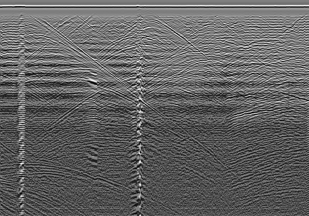
Migrated GPR radargram, Grimsel granite (AU tunnel, MALA GX160 160 MHz)

The granite spine (example 3) runs this chain end-to-end on the real Grimsel ISC data (MALA GX160, AU and VE tunnels, CC-BY-4.0): with the granite_160 preset it extracts 1472 picks on AU and 1485 on VE, at $\mathrm{d}t=0.4464\,\mathrm{ns}$ and $\mathrm{d}x=0.0498\,\mathrm{m}$ (examples/03_gpr_fracture_granite/README.md:14).

Originality. FractureExtractor is evolved-fork. The high-energy + USGS-continuity base is clean-room from the cited literature (USGS Mirror Lake WRIR 99-4018C; Porsani 2006; Isakova 2021, GprFractureExtractComponent.cs:44). The dip-aware shear-count continuity that follows dipping shear zones while gating steep events is the measured delta over the flat-horizon USGS test. Fronted by GPR Fracture Extract (GUID A7E0B0F1-0C0F-4A16-9E3D-0FACE0FACE02, GprFractureExtractComponent.cs:66), Exposure=secondary.

4.3.1 Stone-by-frequency presets¶

GprPresets holds the parameter sets that produced the validated 3-D models, one per stone-type x antenna-frequency, with window sizes as fractions of the trace sample count so a preset transfers across acquisitions (GprPresets.cs:7-25). Two presets are empirically tuned on real data (marble_600 on Bondua Botticino, granite_160 on Doetsch Grimsel); a granite frequency family (25-1200 MHz) and the travertine / andesite / limestone presets carry paper-measured velocities but extrapolated filter windows. The IsEmpirical flag records which is which so the GH component can warn the user (GprPresets.cs:22-24, :86, :111). The marble preset notably narrows the continuity span to 27 traces ($\approx0.65\,\mathrm{m}$) because marble fractures (stylolites, veins) are shorter than granite shear zones ($\approx0.9\,\mathrm{m}$ measured), surfacing marble's genuine short reflectors from the same energy bar (GprPresets.cs:90-94).

Originality. clean-room parameter catalogue, no algorithm. The presets are calibration data; the IsEmpirical honesty flag distinguishes validated from literature-default values.

4.4 From picks to surfaces¶

FractureSurface builds fracture surfaces from picks by two paths (FractureSurface.cs:8-25). The managed loft path extrudes an ordered fracture polyline along strike, or lofts adjacent parallel section-lines across a survey grid onto a common X grid; the surface orientation follows the reflector (sub-horizontal stays sub-horizontal, dipping stays dipping) rather than forcing a vertical sheet (Loft, :42-70; LoftAcrossLines, :77-110). The reconstruct path takes an unordered fracture point cloud and runs geogram screened-Poisson (Kazhdan and Hoppe 2013) first, falling back to CGAL advancing-front for open sheets (TryReconstructFromCloud, :112-139). The heavy 3-D reconstruction is the only place this chapter touches a native shim, and it is optional with a clear error when absent.

Originality. The loft path is clean-room elementary surface construction. The reconstruction path is wrapper-of-native over the geogram (BSD-3, with bundled Kazhdan PoissonRecon MIT) and CGAL (GPL) shims, reached out-of-process; only the dispatch is ours, and the CGAL route is quarantined per the licensing register.

4.5 The uncertainty ladder and safe yield¶

The deliverable is not a fracture surface, it is an honest fracture surface: how far the reconstructed surface can deviate from the true fracture, propagated through the pipeline, so a quarry can set a keep-out margin and pack blocks only into provably-intact rock. FractureUncertainty is that tolerance ladder (FractureUncertainty.cs:6-33). The per-location 1-sigma position uncertainty combines three independent contributions in quadrature:

\[ \sigma_{\text{total}}=\sqrt{\sigma_{\text{recon}}^2+\sigma_{\text{interp}}^2+\sigma_{\text{mesh}}^2}. \]

Reconstruction sigma (original derivation). The GPR time-to-depth conversion $\mathrm{depth}=v\,t/2$ with $v=c/\sqrt{\varepsilon_r}$ has three error sources. First, a relative velocity error that grows with depth: differentiating $v\propto\varepsilon_r^{-1/2}$ gives

\[ \frac{\sigma_v}{v}=\tfrac12\,\frac{\sigma_{\varepsilon_r}}{\varepsilon_r}, \]

so the depth term is $\mathrm{depth}\cdot\sigma_v/v$ (VelocityRelUncertainty, :48-53). Second, the vertical-resolution floor $\lambda/4$, with $\lambda/4=v/(4f)$ (LambdaQuarter, :39-45). Third, the time-zero pick ambiguity $v\,\sigma_{t_0}/2$, where the first-break-to-first-apex window is a rectangular distribution $\sigma_{t_0}=(t_{\text{apex}}-t_{\text{break}})/(2\sqrt3)$ (TimeZeroSigma, RectTimeZeroSigma, :55-65). The combined reconstruction sigma is

\[ \sigma_{\text{recon}}=\sqrt{\bigl(\mathrm{depth}\cdot\tfrac{\sigma_v}{v}\bigr)^2+\bigl(\tfrac{\lambda}{4}\bigr)^2+\sigma_{t_0}^2}. \]

The velocity term leads at quarry depth (Porsani 2006 reports $\pm8.5\text{-}9.5\%$ at 25 m); the time-zero term leads near the surface (Xie, Lai and Derobert 2021); $\lambda/4$ is a floor, not the dominant term (DepthSigma, :67-81). Passing $\sigma_{t_0}=0$ reproduces the original two-term form, so the time-zero rung is an additive evolution of the earlier ladder (:67-72).

Interpolation sigma. Between scan lines the surface is interpolated, and the interpolation has its own uncertainty: zero at a pick, growing in the gaps. This is supplied by the kriging posterior standard deviation. The Kriging class is simple kriging on mean-centred data with a Gaussian covariance $C(h)=\text{sill}\cdot e^{-(h/\text{range})^2}$ and a nugget; the posterior variance at a query point is

\[ \mathrm{var}(x_\ast)=(\text{sill}+\text{nugget})-w^\top w,\qquad w=L^{-1}k_\ast,\quad K=LL^\top, \]

i.e. the prior variance minus what the data explain, via the Cholesky factor (Kriging.cs:19-29). It is the managed replacement for the prototype's scikit-learn GaussianProcessRegressor, exact and shim-free because kriging is linear algebra (Cressie 1993; Rasmussen and Williams 2006).

Mesh sigma. The triangulation cuts the true curved surface by the chord sagitta, $\sigma_{\text{mesh}}=(h^2/8)\,\kappa$ for edge length $h$ and curvature $\kappa$ (MeshSigma, :83-85).

The confidence metric. The optimisation target is not sigma itself but the confidence: the probability that the fracture lies within a fabrication tolerance $T$, assuming a zero-mean Gaussian deviation,

\[ \textsf{confidence}(x)=\operatorname{erf}\!\Bigl(\frac{T}{\sigma_{\text{total}}(x)\sqrt2}\Bigr), \]

averaged over the surface (ConfidenceWithin, :95-100). The error function is the Abramowitz-Stegun 7.1.26 rational approximation ($|\text{error}|<1.5\times10^{-7}$), again to avoid a MathNet dependency (Erf, :222-230). Lowering sigma (calibrate velocity, denser scan lines, higher frequency, finer mesh) raises confidence; the ladder quantifies each trade.

The detection rung (original derivation). A position sigma only matters for a fracture that is seen. A missed fracture has no sigma but is the real yield risk, so the ladder adds a detection model grounded in the imaging literature (Molron et al. 2020 Aspo; Dorn et al. 2012). The minimum detectable area is Fresnel-zone limited and grows with depth, $A_{\min}\approx(\lambda/4)\cdot \mathrm{depth}/2$ above a shallow resolution floor (MinDetectableArea, :111-128). The detection probability factorises over dip, aperture, and size:

\[ P_{\text{det}}=\eta\cdot p_{\text{dip}}\cdot p_{\text{open}}\cdot p_{\text{size}},\qquad p_{\text{size}}=\frac{A}{A+A_{\min}}, \]

with $\eta$ the imaging ceiling ($\approx0.80$ open, Molron; $0.91$ transmissive, Dorn), $p_{\text{dip}}=1$ for sub-horizontal fractures smoothstepping to $0.1$ by $75^\circ$ (surface GPR poorly images sub-vertical fractures), and a sealed-factor penalty for mineral-filled fractures (DetectionProbability, :130-150). The effective confidence caps position confidence by detection completeness, $C_{\text{eff}}=P_{\text{det}}\cdot\textsf{confidence}$, so a low detection probability limits trust however precisely the seen fractures are located (EffectiveConfidence, :152-160; Summarise, :191-220).

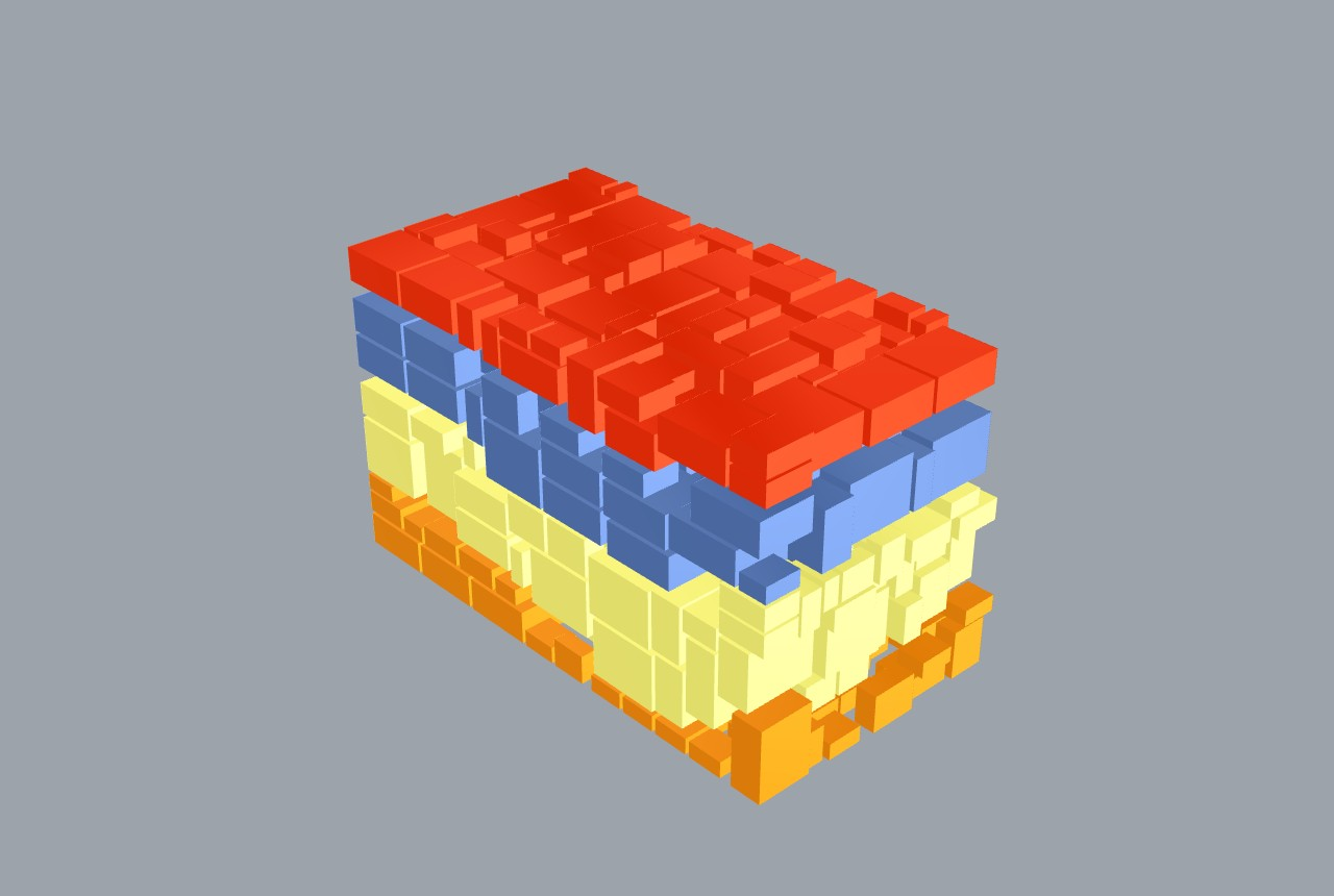
Uncertainty-safe quarry yield: blocks packed only into intact rock, with an inward clearance set to the GPR position sigma

Example 9 is the full quarry decision. The GPR fracture surfaces (from the granite spine) bound the intact zones; Fracture Block Pack (GUID A7E0B0F3-0C0F-4A16-9E3D-0FACE0FACE04) packs fixed-size dimension blocks into each zone with an inward Fracture Clearance wired to the GPR position sigma, so no block sits within the measured uncertainty of a fracture. Toggling uncertainty-safe off gives the optimistic geometric yield; on gives the uncertainty-safe yield (FractureBlockPackComponent.cs:10-25; examples/09_uncertainty_safe_yield/README.md:12-17).

Originality. FractureUncertainty is original-research (A-candidate). The three-rung position ladder, the depth-growing velocity term plus time-zero plus $\lambda/4$ decomposition, and the detection rung with the depth-aware Fresnel floor and the $P_{\text{det}}$ factorisation are the Frahan contribution; the underlying physics is cited (Porsani 2006; Xie 2021; Molron 2020; Dorn 2012). Kriging is clean-room ordinary kriging (Cressie 1993; Rasmussen and Williams 2006). The surface-and-ladder front end is GPR Fracture Surfaces 3D (GUID A7E0B0F2-0C0F-4A16-9E3D-0FACE0FACE03, GprFractureSurface3DComponent.cs:30), which clusters the pick cloud, kriges each fracture, and colour-maps $\sigma_{\text{total}}$ green-to-red.

4.6 RecoveryCascade: multi-scale crack-aware recovery¶

The fracture map feeds the block-cutting solver of chapter 3, but a single-scale packer discards every block a fracture crosses. RecoveryCascade recovers value from those blocks by running the cutter at progressively finer scales: at each scale BlockCutOpt is solved on the region, the non-intersected blocks are recovered, and every cracked block is fed back into the same engine at the next finer scale, cutting around the fracture, until the remnant falls below the smallest marketable size (RecoveryCascade.cs:9-37).

Original derivation: the recovery recursion. The value recovered from a tested region $R$ at scale $s$ is

\[ W(R,s)=\sum_{b\in\text{kept}(R,s)}\!\mathrm{RMV}_s(b)\;+\;\sum_{b\in\text{cracked}(R,s)}\!\begin{cases}W\bigl(\mathrm{AABB}(b),\,s{+}1\bigr) & s{+}1<S,\ \mathrm{Vol}\ge V_{\min}\\[2pt]\text{residual}(b) & \text{otherwise}\end{cases}, \]

where the kept / cracked partition of the winning grid is decided by !bvh.AnyTriangleIntersects against a single shared immutable fracture BVH (RecoveryCascade.cs:25-29, :91-119). The recursion depth is capped at the number of scales, so it cannot run unbounded (:74). Crucially, with a single ScaleSpec the cascade recovers exactly the non-intersected blocks BlockCutOptSolver.Solve finds, with the same winning pose and the same intersection predicate, so it reduces to BlockCutOpt 2020 exactly at scale 1 and is a faithful superset (:21-24). It is grounded in the conditional two-scale (Yarahmadi 2018), usable-leftover (Cherri 2009), and staged-guillotine (Gilmore and Gomory 1965) literatures.

Originality. RecoveryCascade is evolved-fork. The 3-D recursive reject-recover cascade extends the single-scale BlockCutOpt baseline (chapter 3) to which it provably reduces. The header now credits the companion paper (Murugean 2026) for the unified cascade rather than self-labelling "novel"; the earlier unsoftened "novel" wording was flagged E9 in the originality audit (docs/thesis/90_originality.md:188). No GH consumer wires it yet (see Status). The separate FractureBlockPack GH component is a facade-over-primitives self-contained recovery engine that does not call RecoveryCascade, a silent-disagreement risk also tracked in the register.

4.7 Earthworks: bedrock surface and the overburden strip¶

The same GPR picks lift a bedrock surface for the overburden strip. The deepest continuous strong reflector below the weathered cover is the top of fresh rock (Porsani profiles; Bondua bedrock). BedrockSurface.DeepestReflectorPoints reduces a pick set to the deepest qualifying reflector per $(x,y)$ column and converts depth to world elevation $z_r=z_{\text{ground}}(x,y)-\mathrm{depth}$ (BedrockSurface.cs:7-19, :51-93). The picks come from one or more survey lines, scattered in $(x,y)$.

TinMerge.ResampleOntoVertices fuses those sparse bedrock picks onto the dense ground TIN so a downstream prism-difference can compute the overburden volume, because that consumer requires both surfaces sampled on the same triangulation (TinMerge.cs:8-27). It resamples by k-nearest inverse-distance weighting (Shepard 1968):

\[ z(x_\ast)=\frac{\sum_i w_i\,z_i}{\sum_i w_i},\qquad w_i=\frac{1}{d_i^{\,p}},\quad p=2, \]

over the k nearest source picks within a scale-relative radius (a multiple of the median source spacing), with a uniform-grid spatial index, and flags target vertices with no source inside the radius as NaN so the caller can clip them (TinMerge.cs:54-122). Coordinates are recentered first so UTM / quarry-scale $(x,y)$ do not lose mantissa precision (the GeometryNumerics T1 rule, :20-23).

TinPeelFilter is the upstream scan-cleaner. A raw Delaunay or Poisson reconstruction fills the whole convex hull, so concave shorelines and data gaps grow long thin cap triangles and near-vertical gap webs that are not real terrain. The filter iteratively peels border triangles satisfying any of three predicates, then drops connected components below a minimum size (TinPeelFilter.cs:7-29): a long edge $\max(e_0,e_1,e_2)^2>(k\,m)^2$ where $m$ is the median 2-D edge and $k=3$ aggressive / 10 careful; a near-vertical facet with normal tilt $>85^\circ$; and a cap / sliver with an interior angle opposite the border edge $>140^\circ$ (:18-23, ShouldPeel, :139-163). The thresholds are relative to the local median edge, so the same filter works at any survey scale (the scale-relative-epsilon principle).

Originality. TinPeelFilter is clean-room (the border-peel logic ported from the Fade2D land-survey reference's peelOffIf, no upstream code, cited in the Clean Scan Mesh [Algorithm], CleanScanMeshComponent.cs:29-31, GUID A7E0B0F1-0C0F-4A16-9E3D-0FACE0FACE03). TinMerge is clean-room k-NN IDW (Shepard 1968) with a scale-relative radius. BedrockSurface is clean-room: pure reduction and datum shift, no FFT. The bedrock front end is GPR Bedrock Surface (GUID A7E0B0F1-0C0F-4A16-9E3D-0FACE0FACE04, GprBedrockSurfaceComponent.cs:33-35, citing Porsani 2006 / Isakova 2021 for the top-of-rock reflector and Shepard 1968 for IDW).

4.8 The vector counterpart: surface fracture maps¶

GPR sees fractures with depth; a shapefile carries the mapped surface trace network, the cheapest fracture data a quarry has (drone photo plus tracing). Example 26 reads a real ESRI Shapefile of Loviisa rapakivi-granite fracture traces through the Frahan > Quarry > Ingestion vector reader and renders the strike map.

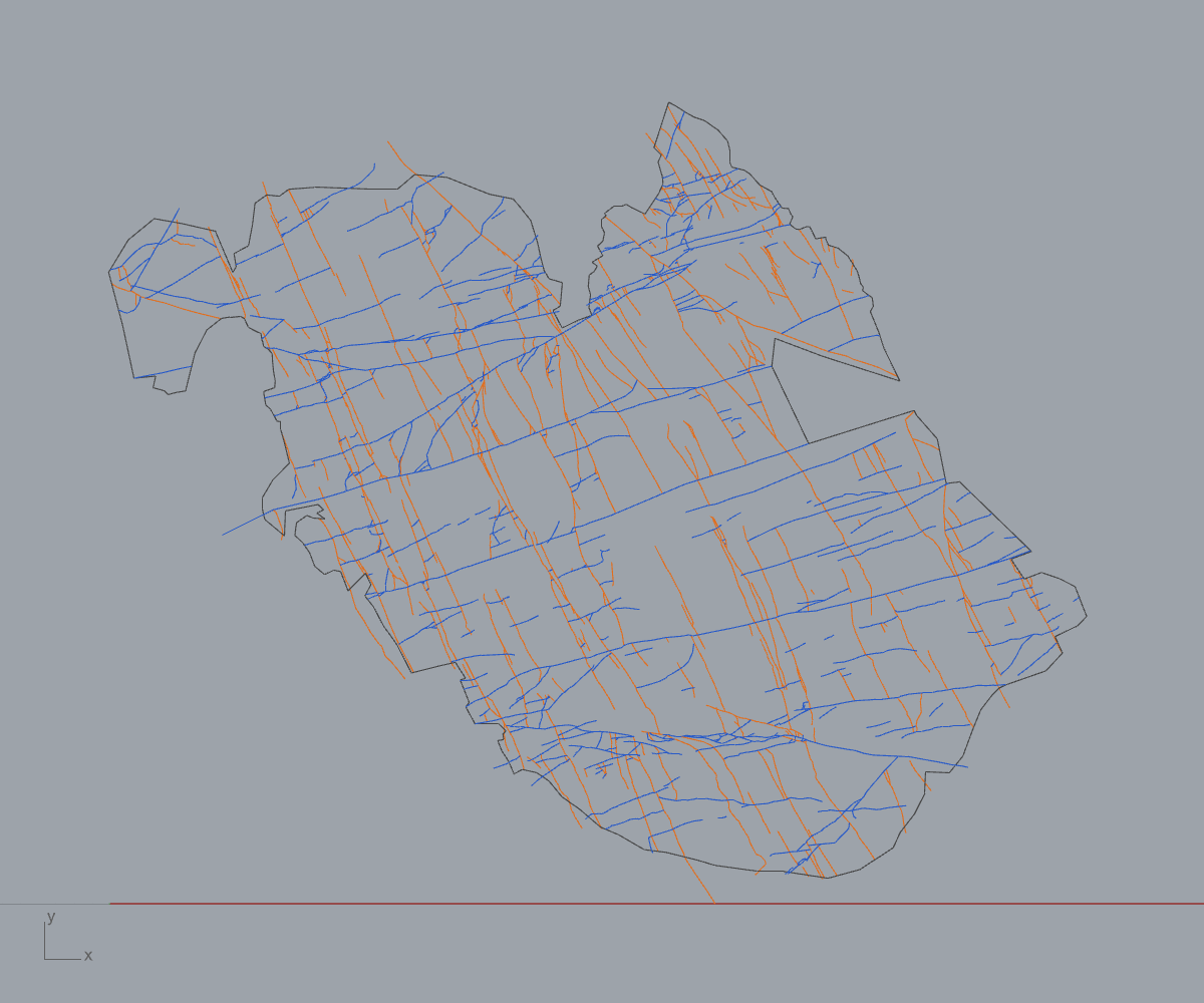
$Loviisa KB11 surface fracture map: 708 traces over a ~54 x 45 m outcrop, coloured by strike set$

The reader returns 708 traces / 6483 vertices, total length 1593.5 m, CRS EUREF_FIN_TM35FIN (EPSG:3067), with two conjugate sets peaking at $\approx15^\circ$ (NNE) and $\approx105\text{-}120^\circ$ (ESE) (Chudasama 2022, CC-BY-4.0; examples/26_loviisa_surface_fractures/README.md:26-30). The strike histogram is the input a quarry needs to orient block cuts away from the dominant joint set, and combined with a GPR depth survey it constrains the 3-D intact-block volume.

Originality. vendored-library reader (NetTopologySuite.IO.Esri, ESRI Shapefile / OGC Simple Features); the strike binning and rendering are clean-room, no new algorithm.

4.9 Status & what's left¶

Example 3 figure is a radargram, not the extracted-pick overlay. The folder ships 03_gpr_radargram_AU.png (the migrated section) plus the two .gh canvases, but no rendered fracture-pick / 3-D surface PNG; the README marks the example "pending live regeneration" with repath, stage groups, and a shaded viewport capture still to do (examples/03_gpr_fracture_granite/README.md:22-26). Severity: medium (documentation / figure gap, the chain itself is validated to the 1472 / 1485 pick counts).
RecoveryCascade has no GH consumer. The recursion is implemented and tested in Core but no canvas component wires it, and the shipped FractureBlockPack component runs its own self-contained recovery engine instead, a silent disagreement risk if the two diverge (docs/thesis/90_originality.md:66, :68). Severity: high.
.gsf is read-only via conversion. Geoscanners AKULA stays unsupported by design; the user must export to SEG-Y with GPRSoft or RGPR first (GprFileReader.cs:46-51). This blocks any dataset that ships only .gsf. Severity: medium (a real Tamil Nadu charnockite data path depends on it).
Literature-default presets are unvalidated end-to-end. Only marble_600 and granite_160 are IsEmpirical=true; the granite frequency family and the travertine / andesite / limestone presets carry paper velocities but extrapolated filter windows (GprPresets.cs:22-24, :110-111). The component warns, but a user running an unvalidated preset gets uncalibrated continuity spans. Severity: medium.
Reconstruction path needs native shims. TryReconstructFromCloud returns a clear error when geogram / CGAL are absent, and the CGAL route is GPL, quarantined out-of-process (FractureSurface.cs:131-138; licensing register E3/E4). The default install has no reconstruction; loft-only surfaces are the fallback. Severity: low (managed loft path covers the common ordered-line case).
AABB child region in the cascade is exact only for axis-aligned blocks. AabbOf is exact for psi-only (axis-aligned) oriented blocks; a fully tilted pose feeds the finer scale a slightly loose axis-aligned bound (RecoveryCascade.cs:122-123). Severity: low (conservative, never drops a real block).

References (this chapter)¶

Stolt, R.H. (1978). Migration by Fourier transform. Geophysics 43(1):23-48. DOI 10.1190/1.1440826. [R146]
Taner, M.T., Koehler, F., Sheriff, R.E. (1979). Complex seismic trace analysis. Geophysics 44(6):1041-1063. DOI 10.1190/1.1440994. [R147]
Cooley, J.W., Tukey, J.W. (1965). An algorithm for the machine calculation of complex Fourier series. Mathematics of Computation 19(90):297-301. DOI 10.1090/S0025-5718-1965-0178586-1.
Porsani, J.L., Sauck, W.A., Junior, A.O.S. (2006). GPR for mapping fractures and as a guide for the extraction of ornamental granite from a quarry. Journal of Applied Geophysics 58:177-187. DOI 10.1016/j.jappgeo.2005.05.010. [R34]
Molron, J., Linde, N., Baron, L., Selroos, J.O., Darcel, C., Davy, P. (2020). Which fractures are imaged with ground penetrating radar? Engineering Geology 273:105674. DOI 10.1016/j.enggeo.2020.105674. [R36]
Dorn, C., Linde, N., Doetsch, J., Le Borgne, T., Bour, O. (2012). Fracture imaging within a granitic rock aquifer using multiple-offset single-hole and cross-hole GPR reflection data. Journal of Applied Geophysics 78:123-132. DOI 10.1016/j.jappgeo.2011.01.010. [R37]
Xie, F., Lai, W.W.L., Derobert, X. (2021). GPR-based depth measurement of buried objects based on constrained least-square fitting. Measurement 168:108330. DOI 10.1016/j.measurement.2020.108330. [R41]
Annan, A.P. (2009). Electromagnetic principles of ground penetrating radar. In: Jol, H.M. (ed.) Ground Penetrating Radar: Theory and Applications. Elsevier, pp 3-40. [R39]
Neal, A. (2004). Ground-penetrating radar and its use in sedimentology. Earth-Science Reviews 66:261-330. DOI 10.1016/j.earscirev.2004.01.004. [R40]
Bondua, S., Monteiro Klen, A., Pilone, M., Asimopolos, L., Asimopolos, N.S. (2024). A set of ground penetrating radar measures from quarries. Data 9(3):42. DOI 10.3390/data9030042. [R44]
Huber, E., Hans, G. (2018). RGPR — an open-source package to process and visualize GPR data. 17th International Conference on GPR, IEEE. DOI 10.1109/ICGPR.2018.8441658. [R43]
Lucius, J.E., Powers, M.H. (1999). USGS Open-File Report 02-166: GPR data-format documentation (pulseEKKO DT1/HD spec). [R45]
Shepard, D. (1968). A two-dimensional interpolation function for irregularly-spaced data. Proc. 23rd ACM National Conference, pp 517-524. DOI 10.1145/800186.810616.
Cressie, N.A.C. (1993). Statistics for Spatial Data. Wiley. DOI 10.1002/9781119115151. [R119]
Rasmussen, C.E., Williams, C.K.I. (2006). Gaussian Processes for Machine Learning. MIT Press. DOI 10.7551/mitpress/3206.001.0001. [R120]
Kazhdan, M., Hoppe, H. (2013). Screened Poisson surface reconstruction. ACM Transactions on Graphics 32(3):29. DOI 10.1145/2487228.2487237. [R91]
Yarahmadi, R., Bagherpour, R., Taherian, S.G., Sousa, L.M.O. (2018). Discontinuity modelling and rock block geometry identification to optimize production in dimension stone quarries. Engineering Geology 232:22-33. DOI 10.1016/j.enggeo.2017.11.006. [R20]
Cherri, A.C., Arenales, M.N., Yanasse, H.H. (2009). The one-dimensional cutting stock problem with usable leftover. European Journal of Operational Research 196:897-908. DOI 10.1016/j.ejor.2008.04.039. [R12]
Gilmore, P.C., Gomory, R.E. (1965). Multistage cutting stock problems of two and more dimensions. Operations Research 13:94-120. DOI 10.1287/opre.13.1.94. [R11]
Chudasama, B. (2022). Loviisa rapakivi-granite fracture and lineament dataset, southern Finland. Zenodo, CC-BY 4.0. [R53]
Murugean, L. (2026). GPR-to-block-yield optimization for fractured dimension-stone quarries (submitted, Bulletin of Engineering Geology and the Environment; reproducibility deposit). DOI 10.5281/zenodo.20608279. [R144]
USGS (1999). Mirror Lake GPR continuity protocol, Water-Resources Investigations Report 99-4018C (>=40-trace lateral-continuity criterion).
Isakova, E. (2021). GPR survey of fractured Karelia granite (OKO-2, 150 / 1200 MHz antennas).