Chapter 0 — Repository Overview and Cross-Cutting Foundations

Author: Independent Research. Open data, open source. No university affiliation.

This chapter states what Frahan StonePack is, how the assemblies are layered, what the ribbon offers, and the shared numeric foundations that every algorithm in later chapters stands on. The conventions follow AGENTS.md: a result is true only when visually validated in Rhino (criterion c); numbers from the headless harness are measured, not validated, until seen on the canvas.

---

0.1 What the project is

Frahan StonePack is a pre-CAM stone fabrication-readiness bridge for Rhino and Grasshopper. It sits between design intent and machine-ready fabrication. It is not a CAM system and does not generate toolpaths as its product. It answers the questions a CAM package assumes are already solved for natural stone: which block out of this quarry, cut on which planes, in which order, oriented how, packed against which neighbours, and stable under gravity once set. The output is a fabrication-ready geometric plan with stone metadata attached, which a downstream CAM or robotic-setting stage then consumes.

The project carries two design flows as first-class citizens.

• Top-down (form-first). A target form is given, and the system finds or cuts the stone to realise it: voussoirs for an arch or vault, a sculpture decomposed into masonry-scale blocks, a quarry block cut to yield a designed shape. Imposition of intent onto material.
• Bottom-up (material-first). The stock is given, and the form emerges from it: random rubble walls, vein-flow and live-edge selection, Trencadis mosaics from fragments. Negotiation with material.

The application domain is dimension and monument stone, with a working emphasis on granite (Tamil Nadu deposits, where joints in poorer rock drive the GPR ambition) and on marble and limestone for the bench-to-block yield studies. The spine runs from sub-surface sensing through to a setting plan, so the same repository carries ground-penetrating-radar fracture mapping, LiDAR and photogrammetry ingest, mesh reconstruction, 2D and 3D packing, masonry assembly with contact equilibrium, and fabrication export.

---

0.2 Assembly and layer architecture

The solution under src/ is layered so that the algorithmic core never depends on Rhino. This keeps the math headless-testable and lets the same engine run inside Rhino, inside a benchmark harness, or inside an out-of-process worker.

Assembly	Target	Role
Frahan.StonePack.Core	net48, Rhino-free	All geometry and solver math. Plain double arrays and Frahan-owned structs (Vec3, Size3, Box3). 11 sub-namespaces.
Frahan.EdgeMatching.Core	net48, Rhino-free	Fragment edge-matching and reassembly (boundary rails, projection bootstrap, soft-ICP / L-BFGS).
Frahan.Kintsugi.Port	net48, Rhino-free	Learned 6-DoF fracture-reassembly port with a verifier gate (see licensing note below).
Frahan.RubblePack	net48	Multi-bin rubble packing front end.
Frahan.StonePack.GH	net48, Grasshopper	The facade. Converts RhinoCommon to Core types at the component edge, calls Core, converts back. Builds to ONE Frahan.StonePack.gha.
Frahan.StonePack.Rhino	net48, RhinoCommon	Rhino plug-in surface (commands, document hooks).

The boundary rule is strict and load-bearing for the thesis claim of clean, reusable math. The Core takes no using Rhino. Components in the GH layer translate at their input/output edge only. This is why the packing benchmarks (--packbench, --pack2dstudy) and the unit tests run with no Rhino present, and why the same BlockCutOptSolver is the baseline the research chapters evolve rather than a re-implementation.

Native bridges are reached through a lazy boundary, not a hard link. The default install ships no native DLL. NativeBridge.cs and NativeBackendLoader probe a fixed search path on first use, fall back to a managed default with a surfaced remark if the DLL is absent, and never throw on a missing backend. The FRAHAN_BACKEND environment variable forces a specific backend for testing. The native shims live under native/ and are reached via P/Invoke:

Bridge	Library	License	What it does	Citation
nfp_kernel	Clipper2 (vendored, unmodified)	BSL-1.0	Batched No-Fit-Polygon Minkowski sums for the 2D nester; one native call per part replaces the managed Clipper2 loop. Measured ~8x wall-time on the 7-shield bench.	(Johnson, Clipper2)
Clipper2 (managed)	Clipper2 adapter	BSL-1.0	Vatti-derived polygon clipping for 2D Boolean and overlap validation.	(Johnson, Clipper2)
cgal_shim	CGAL Polygon Mesh Processing	GPLv3 / commercial	Robust non-convex mesh-mesh Boolean (corefinement, EPECK/EPICK hybrid), straight skeleton, SDF segmentation, heat-method geodesics, PMP repair.	(CGAL PMP)
geogram_shim	Geogram v1.9.9	BSD-3	Mesh repair, hole filling, remesh and decimation, restricted Voronoi, constrained Delaunay tetrahedralisation, and bundled Poisson reconstruction.	(Levy, Geogram; Kazhdan, Bolitho & Hoppe 2006)
BFF	Boundary First Flattening	as published	Conformal surface flattening for surface mosaicing, with a Frahan-original chart-scale recovery.	(Sawhney & Crane 2017)

Licensing note. CGAL Polygon Mesh Processing is GPLv3 (or commercial). Anything that links it inherits that obligation. The architecture quarantines this risk: CGAL is reached only through the out-of-process shim and is absent from the default install, so the shipped managed assemblies do not link GPL code. The same out-of-process routing is also required for stability, because in-process CGAL or geogram Boolean can crash Rhino (AGENTS.md §3). Geogram (BSD-3) and Clipper2 (BSL-1.0) are permissive and carry no copyleft obligation. The Kintsugi port carries a separate, flagged licensing question recorded in the originality audit and is kept in its own assembly for that reason.

---

0.3 The ribbon: 18 tabs

The plug-in publishes one Frahan ribbon. Sub-categories partition the 206 shipped GH_Component types into 18 tabs. Counts below are component placements per ("Frahan", "<tab>") category attribute.

#	Tab	Count	Role (one line)
1	Quarry	43	Quarry-scale block-cut optimisation: GPR-aware yield, BlockCutOpt solver, recovery cascade, georeferenced cutting.
2	Masonry	35	Wall and shell assembly: rubble and ashlar packing, polygonal masonry, contact equilibrium (CRA / RBE).
3	Lab	26	Experimental and utility nodes; each cross-references a primary node (no dead ends).
4	Mesh	25	Mesh hygiene and operations: clean, remesh, decimate, Boolean, segment, heightmap.
5	2D Packing	13	Sheet and slab nesting: NFP bottom-left-fill, hole-aware contact nesting, irregular sheet fill.
6	Fabricate	11	Fabrication export: wire-saw toolpath adapter, stone-cut metadata, cut sequence and export.
7	Fracture	10	Fracture-pattern generation and Voronoi fracture planes for block and slab zoning.
8	EdgeMatch	10	Fragment reassembly: boundary-rail matching, segment extraction, solve and options.
9	3D Packing	9	Volumetric packing: block-pack tree, drop-settle, mesh-accurate placement.
10	Kintsugi	7	Learned 6-DoF fracture reassembly with verifier gating.
11	Voussoir	5	Voussoir generators: arch and pendentive-vault cell factories, pack-into-block.
12	Trencadis	5	Mosaic-from-fragment placement, physics and edge-match variants.
13	Ingest	5	Format readers: vector, point cloud (E57, LAS/LAZ), CAD, raster, GPR.
14	Surface Packing	4	Pack onto a curved surface via BFF flattening and barycentric mapping.
15	Slab	4	Slab-cut operations from a bench, CGAL-backed.
16	Sculpt	3	Fit a form into a block, sculptor-output branch.
17	Reports	3	Cost, volume and plan reporting; LaTeX and table emission.
18	Analysis	3	Boundary-rail indexing and geometric analysis helpers.

The per-tab counts above sum to 221, which exceeds the 206 unique GH_Component types: the 221 figure counts category-attribute placements (a component can register under more than one sub-category, or appear in Lab as well as its home tab, and is then counted once per placement), while 206 is the count of distinct GH_Component types. A third number is the source-file count: a grep for : GH_Component / : GH_TaskCapableComponent over src/Frahan.StonePack.GH matches 174 .cs files, fewer than the 206 types because several files declare more than one component class (for example BlockCutOptComponents.cs, CgalTestComponents.cs, and GeogramTestComponents.cs each hold a family of components). So the three figures are distinct by construction: 174 source files, 206 unique component types, 221 category placements.

The ribbon obeys the canvas rules in AGENTS.md §6: one canonical type per concept, no ghost components (every node on the primary ribbon emits a real valid output), and heavy nodes carry a default-false Run gate so the canvas stays responsive. Monolith ("monster") components are facades over published primitives, never black boxes, and ship a composed-equivalent .gh beside them.

---

0.4 Shared numeric-hygiene foundations

A single defect recurred across nine of the top ten audited algorithms: geometry computed in raw world coordinates loses precision, and fixed absolute epsilons are meaningless at architectural scale. The fix is identical everywhere, so it lives once in Frahan.Masonry.Geometry.GeometryNumerics and is reused throughout. Three rules, then a tolerance budget, then a units table.

0.4.1 Recenter to centroid

Quarry and UTM coordinates run at \(10^5\) to \(10^6\) mm. IEEE-754 double has about 15 to 16 significant decimal digits, so working at \(10^6\) leaves only 9 to 10 digits below the unit, and any sub-millimetre geometry decision is made on noise. The remedy is to translate to the centroid before computing and add it back on emit.

Given vertices \(\{p_i\}_{i=1}^{n}\) with \(p_i \in \mathbb{R}^3\), the centroid is

\[\bar{p} = \frac{1}{n}\sum_{i=1}^{n} p_i,\]

and the recentred set is \(p_i' = p_i - \bar{p}\). Every result \(q'\) is emitted as \(q = q' + \bar{p}\). This is a pure translation, so it is exact for the algorithm (an isometry preserves all distances and angles) while recovering full float64 precision near the origin. The implementation is GeometryNumerics.Recenter, which returns the shifted copy and the centroid to add back.

0.4.2 Scale-relative epsilon

A tolerance must mean the same thing whether the model is in millimetres or in metres. Let \(L\) be the natural scale of the point set, taken as the bounding-box diagonal

\[L = \sqrt{(x_{\max}-x_{\min})^2 + (y_{\max}-y_{\min})^2 + (z_{\max}-z_{\min})^2}.\]

The scale-relative epsilon is

\[\epsilon = \max(\text{floor},\; c \cdot L),\]

where \(c\) is a small dimensionless base tolerance and \(\text{floor}\) is an absolute minimum that prevents collapse to zero on a degenerate (near zero-extent) input. In code this is ScaleRelativeEpsilon(baseEps, scale) = baseEps * max(|scale|, 1), taking \(\text{floor} = \texttt{baseEps}\) via the \(\max(\cdot, 1)\) guard and \(c = \texttt{baseEps}\) against \(L\). The matching near-equality test is relative at any magnitude:

\[|a - b| \le \epsilon \cdot \max\!\big(1,\, |a|,\, |b|\big).\]

A related guard protects the integer-coordinate Boolean path. Clipper2 works in Int64, so a vertex scaled by a fixed \(10^6\) can overflow at quarry scale. After recentring, the safe integer scale is

\[s = \min\!\Big(s_{\text{req}},\; \frac{m \cdot \texttt{Int64.Max}}{|x|_{\max}}\Big),\]

with margin \(m \approx 0.01\), implemented as SafeIntegerScale. Recenter first so \(|x|_{\max}\) is the local extent, not the world position.

0.4.3 The tolerance budget

A pipeline must run one reconciled tolerance system, not several unreconciled ones. From a single model absolute tolerance \(t\) and the scale \(L\), the budget derives all members scale-relative, where \(m = \epsilon(t, L)\):

\[t_{\text{model}} = m,\quad t_{\text{join}} = 10\,m,\quad t_{\text{intersection}} = 0.1\,m,\quad t_{\text{snap}} = 0.01\,m.\]

Join is looser because vertex and edge welding should tolerate more drift; intersection is tighter because Boolean and clip decisions must be crisp; snap-rounding sits below intersection. This is ToleranceBudget.From in GeometryNumerics. Multipliers are tuned per algorithm, but the source is always one value.

For fabrication, the geometric tolerance must stay safely inside the kerf, otherwise rounding can place a cut where the saw physically cannot land. The committed rule is

\[\epsilon_{\text{geo}} < \frac{\text{kerf}}{3},\]

with kerf treated as a process constant carried separately from \(\epsilon_{\text{geo}}\) (a typical quarry kerf is \(0.05\) m). Clearance between placed parts is a function of size and process, not a fixed constant:

\[\text{clearance} = f(L, P),\]

so a 50 cm voussoir and a 5 cm shard get different joint budgets at the same relative honesty. Empirically the joint residual budget scales with the carving process: cathedral voussoirs are CNC-finished to roughly 0.1 to 0.2 mm (Quarra Emanuel 9 field tolerance), so their joint target sits near 2 mm; hand-fragmented Trencadis shards are robot-placed at about 0.05 mm repeatability but the shard edge is mm-rough, so the joint target relaxes to about 5 mm. The edge-matching core carries this as a scale-relative gate (residual factor times the shape scale), which is why a fixed absolute residual is the wrong default.

0.4.4 Units per application

World coordinates default to metres, the engineering-model convention in Rhino. The shop side works in millimetres. The mismatch is real and has bitten fixtures before, so the per-application table is explicit and the GH facade converts at the component edge.

Application	World unit	Standard dimension (example)	\(\epsilon_{\text{geo}}\) regime	Kerf / process constant
Site / quarry / bench	m	bench 5650 x 5675 m study area; block 3 x 1.5 x 1.5 m	\(\max(\text{floor},\, c L)\), \(L\) = bench diagonal	kerf 0.05 m
Slab / dimension stone	m	slab 3.2 x 2 m	scale-relative on slab diagonal	gangsaw / wire-saw kerf
Masonry assembly	m	wall multi-m; rubble and ashlar	scale-relative on wall extent	dry-set, no kerf; clearance = f(L)
Mosaic / Trencadis	mm	tile field ~1100 mm, grout ~5 mm	scale-relative on shard span	hand-fragment; joint ~5 mm
Monument	m	monument 1.2 x 1.2 x 3.5 m	scale-relative	carving tool diameter
Vessel / artefact	mm	vessel ~100 x 280 mm	scale-relative	mill tool diameter
Shop / secondary cut	mm	converted to m on entry	\(1\) nm dedupe, \(10^{-12}\) SAT	sawblade radius (mm)

Two helpers convert between metres and the active Rhino document unit (ToRhinoUnit, MmToMetres / MetresToMm), and the secondary-cut planner converts mm input to metres on entry so downstream yield metrics stay in \(\text{m}^3\) across scales. Note the historical fixture trap: a default File3dm is in millimetres, so geometry authored at metre magnitudes can land 1000x small. The cards layer fixes this at fixture creation.

---

0.5 The data-flow spine

Every workflow in this repository, top-down or bottom-up, is a path through one spine:

ingest → process → segment → pack/cut → stabilise → fabricate.

• Ingest. A reader pulls the raw source into Rhino-side or Core-side geometry: GPR radargrams, LiDAR and photogrammetry point clouds (E57, LAS/LAZ), CAD vector, raster, mesh. The Ingest tab plus the ScanIngest namespace own this stage. Heavy point clouds are voxel-downsampled and chunked; multi-million-vertex meshes are never internalised in a saved .gh.
• Process. Sensing and mesh hygiene turn raw evidence into usable geometry: GPR f-k migration and fracture extraction, Poisson or CGAL reconstruction, hole filling, remesh and decimate. The Mesh tab and the geogram and CGAL shims serve here.
• Segment. The clean geometry is partitioned into fabrication units: fracture-aware zoning, Voronoi fracture planes, SDF or sharp-edge mesh segmentation, sculpture-to-blocks decomposition.
• Pack / cut. The core optimisers place or cut: 2D nesting (NFP bottom-left-fill and hole-aware contact nesting), 3D block-pack with drop-settle, BlockCutOpt quarry cutting with the recovery cascade, voussoir packing. This is where the measured yield claims live and die against --packbench and --pack2dstudy.
• Stabilise. Placed assemblies are checked and settled: drop-settle physics, centre-of-mass over support, contact equilibrium (CRA / RBE) for masonry. A wall that does not stand is not a result.
• Fabricate. The plan is emitted machine-aware: wire-saw toolpath adapter, georeferenced cutting planes and marking, stone-cut metadata, cut sequence, export. This is the hand-off to CAM, not CAM itself.

The recenter, scale-relative epsilon, and one-tolerance-budget rules of §0.4 apply at every stage, which is what makes a pipeline spanning seven orders of magnitude of physical scale (mm shard to km outcrop) numerically honest end to end.

---

0.6 Representative outputs

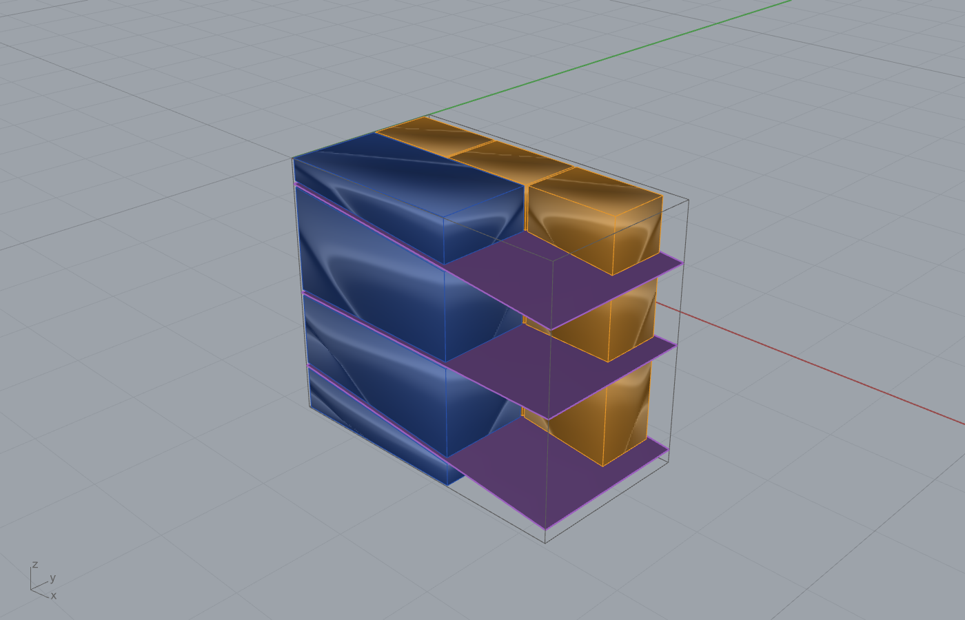
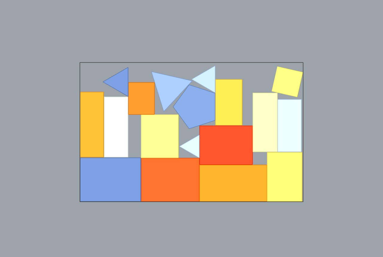
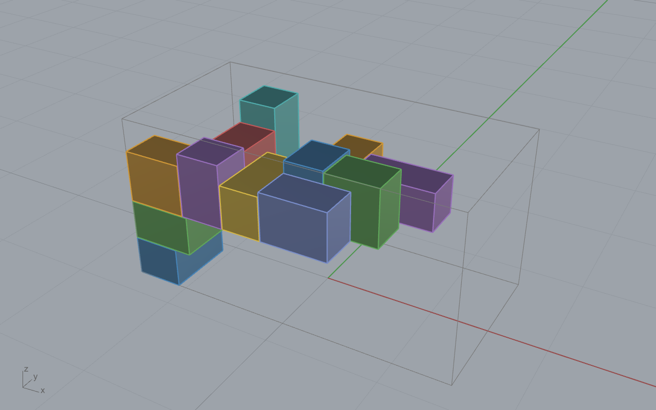
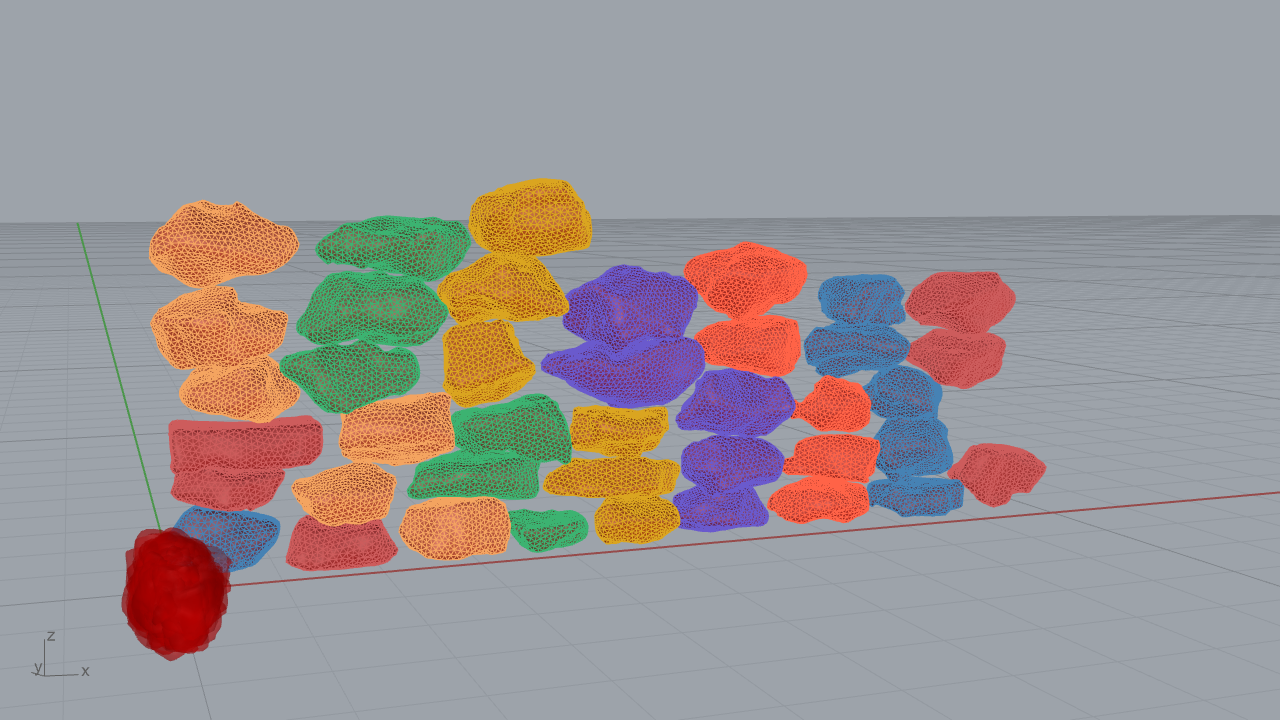
These are git-tracked example renders that exercise the spine across both design flows. Each is the visually validated form (criterion c), produced on the canvas, not by an external bake script.

Top-down cutting and yield (process → segment → pack/cut → fabricate):

2D and 3D packing (pack/cut):

Bottom-up masonry assembly (segment → pack/cut → stabilise):

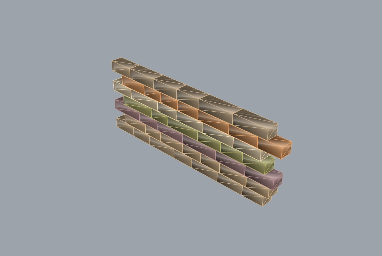
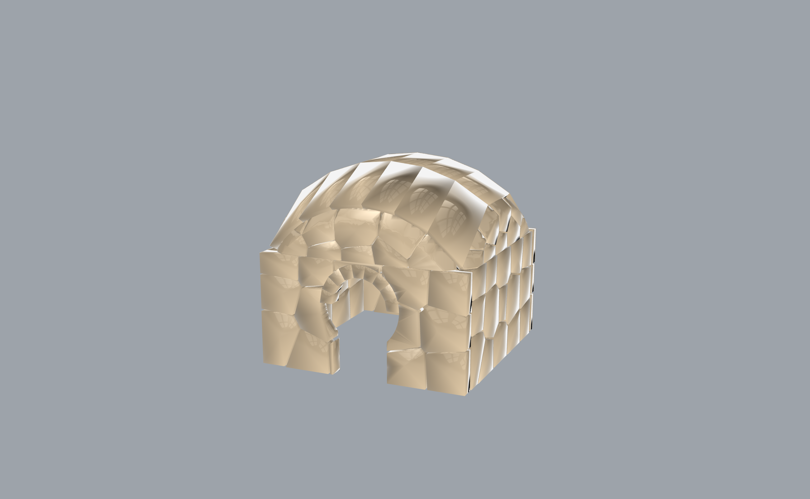
Polygonal masonry at building scale (top-down form, contact-stable):

---

References

• CGAL Polygon Mesh Processing. GPLv3 / commercial. https://doc.cgal.org/latest/Polygon_mesh_processing/
• Johnson, A. Clipper2. BSL-1.0. Vatti-derived polygon clipping. https://github.com/AngusJohnson/Clipper2
• Kazhdan, M., Bolitho, M. & Hoppe, H. (2006). Poisson surface reconstruction. Eurographics Symposium on Geometry Processing. (Bundled inside Geogram as GEO::PoissonReconstruction.)
• Lévy, B. Geogram v1.9.9. BSD-3. INRIA / ALICE. https://github.com/BrunoLevy/geogram
• Sawhney, R. & Crane, K. (2017). Boundary First Flattening. ACM Transactions on Graphics 36(4):109. DOI 10.1145/3072959.3056432.